MImapqtl Options

Table 3.8 shows the command line options specific to MImapqtl.

Table 3.8: Command Line Options for MImapqtl

Option	Default	Explanation
-i	qtlcart.cro	Data File
-o	qtlcart.mim	Output File
-e	qtlcart.log	Error File
-m	qtlcart.map	Genetic Linkage Map File
-E	qtlcart.eqt	Initial model file
-O	qtlcart.mqt	Output model file
-s	1590337669	Random Number Seed
-t	1	Trait to analyze
-q	19	Maximum number of QTL to fit
-k	19	Maximum number of epistatic interactions
-d	2.000000	Walking speed in cM
-S	1	Information criterion [1-6]
-L	0.000000	Threshold for adding/dropping parameters
-I	smprtSeC	Work code
-p	0	Phase of analysis

If you choose to begin analysis from some initial model, it should be formatted as an Rqtl output file and specified with the -E option. For data sets with multiple traits, you can specify the trait to analyze with the -t option. If the specified trait is 0, then all traits whose names begin with a plus sign ($+$) will be analyzed (one at a time). If the specified trait is larger than the number of traits, then all traits will be analyzed one at a time, unless their names begin with a minus sign ($-$).

You may specify a maximal number of QTL and epistatic interactions to fit in the model. The limitations of C on a 32 bit computer mean that you can only fit up to 19 QTL in a cross with three marker genotypes (SFx and RFx lines). Thus, 19 will be a hard limit on the number of loci at this time. In practice, it is not wise to try to fit more than $2\sqrt{n}$ parameters, where $n$ is the sample size. Thus, MImapqtl will automatically adjust this number so that it is no greater than $2\sqrt{n}$ for backcrosses and recombinant inbred lines, $\sqrt{n}$ for lines with three marker genotypes (since each QTL has an additive and a dominance effect). Once main effects are fitted for the QTL, MImapqtl searches for epistatic effects. Again, it will only try to fit up to $2\sqrt{n}$ parameters so only $2\sqrt{n}$ minus the number of main effects will be fitted. For example, if you have a sample size of 400, then $2\sqrt{n} = 40.$ For an SF2 line, if you find 10 QTL, then 20 parameters have been fitted (10 additive and 10 dominance effects). Thus, there will be up to $40 - 20 = 20$ possible epistatic effects that can be fitted.

The walking speed is identical to that in Zmapqtl and JZmapqtl and is used during the refinement of QTL positions and the search for new QTL. For the refinement of QTL position, for each QTL, the position is moved within the QTL interval from one end to the other and an information criterion is calculated for each position. The minium over the interval is the best position for the QTL.

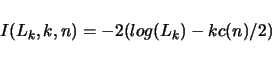
The information criterion is is a function of the likelihood ratio and the number of parameters that gives an indication of how good the model fits the data. This is a function in form

$$I(L_k,k,n) = -2(log(L_k) - k c(n) / 2)$$

where $L_k$ is the likelihood for a $k$ parameter model and $c(n)$ is a penalty function and $log$ is the natural log function. The penalty function $c(n)$ takes one of six forms:

1. $c(n) = log(n)$ [SchwarzSchwarz1978]

2. $c(n) = 2$ [AkaikeAkaike1969]

3. $c(n) = 2 log(log(n))$ [Hannan and QuinnHannan and Quinn1979]

4. $c(n) = 2 log(n)$ [BromanBroman1997]

5. $c(n) = 3 log(n)$ [BromanBroman1997]

6. $c(n) = 0$

Use the numbers above with the -S option to indicate which information criterion you want to use. When comparing a model with $k$ parameters to one with $k-1$ parameters, if $I(L_{k-1},k-1,n) - I(L_k,k,n)$ is greater than the threshold value specified with the -L option, then the parameter is considered significant. During a scan over the entire genome, if the maximum of $I(L_{k-1},k-1,n) - I(L_k,k,n)$ is greater than the threshold, then that position parameter is retained. A non-zero penalty function supersedes the requirement of a true threshold. Therefore, if using one of the first five penalty functions, you can use a threshold of 0.0. For function six (that is, no penalty), it is best to do a permuation test to determine the initial threshold.

In general, it is probably best to start with information criterion 1 with a threshold of 0.0. We have done some initial simulations to support the utility of this approach. If no QTL are identified using information criterion 1, then one could use no penalty function and do a permutation test for the threshold.