Given a genetic linkage map, Rqtl can place a random set of quantitative trait loci on the map. The program simulates the positions and effects (additive, dominance and epistatic) of the QTL. It can also reformat a given set of QTLs defined in an input file of filetype ``qtls.inp'' that is explained in Section 6.2.1. The given set of QTLs might be made up by the user, or a set of estimates from a previous analysis of a data set. Table 2.3 presents the command line options for Rqtl. The default values from the table tell Rqtl to simulate nine QTLs for one trait.
For simulations, the user can specify the average number of QTLs per trait,
the number of traits, and parameters for dominance and additive effects. Epistatic effects are simulated with
the same parameters used for the dominance effects. We use the
convention that ![]() alleles are from for
alleles are from for ![]() lines and
lines and ![]() from
from ![]() lines.
lines.
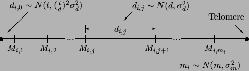
The output file encodes QTL with their positions and effects. A QTL is defined with a line beginning in ``-l'' and followed by its number, chromosome, left flanking marker, two recombinatin fractions and its additive and dominance effects. Here is an example of a set of simulated QTL:
-k     2   for trait -number  1
#      #  ..Chrom..Markr.  .RecombiL.  .RecombiR.  .Additive.  .Dominance
-l     1      2      9       0.0477      0.0475      0.2326      0.0000
-l     2      3      8       0.0906      0.0001      0.1687      0.0000
QTL number 1 is on chromosome 2 following marker number 9. Marker 9 is thus the left flanking marker and has a recombination frequency with the QTL of 0.0477. The right flanking marker would be marker 10 on chromosome 2, and it has a recombination fraction of 0.0475 with the QTL. Figure 2.5 graphically illustrates how QTL positions are encoded. QTL number 1 in the above example has an additive effect of 0.2326 and no dominance.
Dominance can take on the values 1, 2, 3 or 4. 1 means no dominance, while 2
means ![]() is dominant and 3 means
is dominant and 3 means ![]() is dominant. A value of 4 means that
dominance for each QTL will be random in magnitude and sign. The degree of
dominance will be a Beta random variable
is dominant. A value of 4 means that
dominance for each QTL will be random in magnitude and sign. The degree of
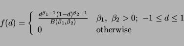
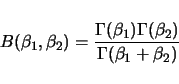
dominance will be a Beta random variable ![]() with shape parameters
with shape parameters
![]() . The density function for
. The density function for ![]() is
is
 |
(2.5) |
 |
(2.6) |
Epistatic effects are generated from the same distribution as the dominance effects.
For a ![]() QTL model, there are
QTL model, there are ![]() potential dominance effects. For each unordered pair of
loci, there are Additive by Additive, Additive by Dominance, Dominance by Additive and
Dominance by Dominance terms, and thus
potential dominance effects. For each unordered pair of
loci, there are Additive by Additive, Additive by Dominance, Dominance by Additive and
Dominance by Dominance terms, and thus ![]() possible epistatic interactions. Only a proportion
of these will be nonzero, with that proportion specified by the -E option.
The proportion should be in the range
possible epistatic interactions. Only a proportion
of these will be nonzero, with that proportion specified by the -E option.
The proportion should be in the range
![]() .
.
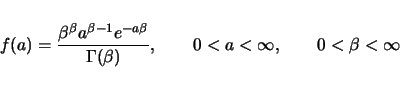
The additive effects of the QTLs are independent, identically distributed
random variables sampled from the gamma distribution
[ZengZeng1992, page 993, equation 12] and reprinted here:
If an input file is specified, then it is translated into a format readable by Rcross and the options in Table 2.3 from ``Number of Traits'' and below are ignored. The input file format ``qtls.inp'' is defined in Section 6.2.1. This input file format will allow a wide variety of genetic models to be simulated.